Using Black-Scholes Model to evaluate Structured Warrants

Black-Scholes model was developed by Fischer Black and Myron Scholes in 1973.  It is a mathematical model of a financial market containing derivative investment instruments (Read more here).  It is widely used, often with adjustments, to determine the price of options.

There are many types of derivative options in the market.  One of the most popular derivative options in Bursa Malaysia are the Structured Warrants (Read more here).  Today, I am going to discuss the usage of Black-Scholes model in Structured Warrants evaluation.

To construct a simple Black-Scholes model using excel, one can refer to this link.  I did some modification on the model in order to fit the characteristics of the structured warrants available in Bursa Malaysia.

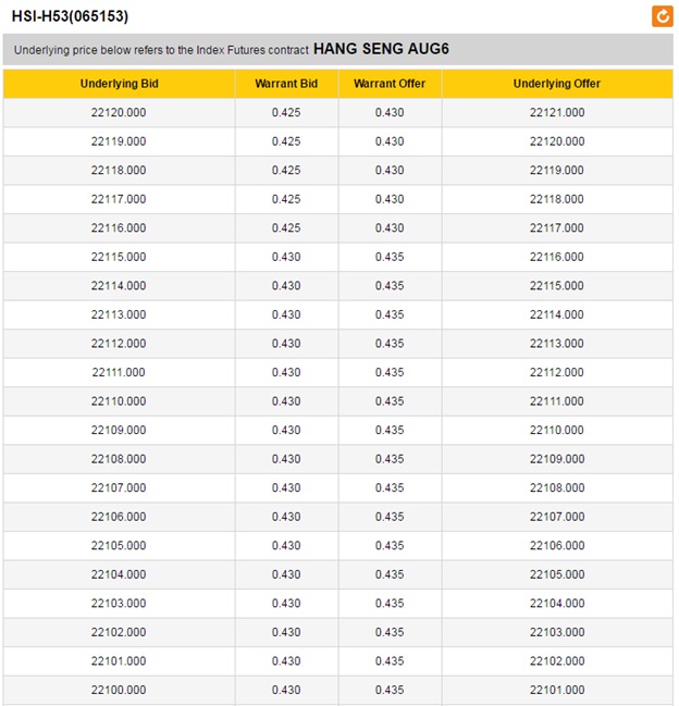
The following table (Table 1) is the structured warrants price of the HSI-H53 as at 26-Jul-16.  To check the accuracy of the model, it is compared with the offer price by the issuer (Table 2).  This model was tested on other structured warrants as well; the accuracy is always within the spread of the structured warrants.

Table 1

Future Index	Black-Scholes Model HSI-H53 price
22120	0.429
22110	0.431
22100	0.432
21880	0.433

Table 2

The following snapshot (Picture 1), is the Black-Scholes model in excel format.  (Readers who are interested to construct the Black-Scholes model using Excel spreadsheet can contact me via email.  Private tutorial or class can be arranged.)

Picture 1

There are few variables that affect the structured warrant price.  The most significant factor is the underlying stock price.  In this example, it is the Hang Seng Future Index.  The following table (Table 3) shows the impact of Hang Seng Future Index changes to the HSI-H53 price.  Every 1% changes of the Hang Seng Index with cause the HSI-H53 price to fluctuate about 6%.

Table 3

Future Index	Put Option Price	Percentage changes of Index	Percentage changes of Put Option Price
23205	0.313862973	5.00%	-27.31%
22984	0.334834542	4.00%	-22.46%
22763	0.357055027	3.00%	-17.31%
22542	0.380583676	2.00%	-11.86%
22321	0.40548107	1.00%	-6.10%
22100	0.431809	0%	0%
21879	0.459630311	-1.00%	6.44%
21658	0.489008773	-2.00%	13.25%
21437	0.520008864	-3.00%	20.43%
21216	0.552695579	-4.00%	28.00%
20995	0.587134208	-5.00%	35.97%

The second significant factor that will impact the option price is the holding period.  In option trading, “buy and hold” strategy is “No”, “No”, “No”.  Because it is very important, so have to say it three times.  The following table (Table 4) shows the holding period impact of the put option.

Table 4

Hang Seng Future Index	Holding Duration	Warrant Price	%
22100	0	0.431	0
22100	3	0.422	-2.09%
22100	5	0.416	-3.48%
22100	10	0.399	-7.42%
22100	14	0.386	-10.44%

  

From the table we can see that, even the underlying Hang Seng Future Index stays constant, by holding the put option for 3 days, the option price will automatically reduce by 2.09%.  As such, in side way market, where the Index stay about the same level for long period of time, eventually the option price will diminish to zero value.

There is another important variable in Black-Scholes model, which is the implied volatility.  This is the most difficult variable to determine.  There are many ways to estimate but for now, the easiest way is to use the implied volatility rate provided by the structured warrants issuer.

In summary, traders who are interested in structured warrants trading can use the Black-Scholes model to evaluate the risk and return.  The key principle is – Do not apply “buy and hold” strategy on option trading.  Unless the option is deep in the money and the trader is ready to exercise the option on maturity.  That will be discussed in another article.

Disclaimer:  The above option price calculations do not imply any buy or sell recommendation.   The author disclaims all liabilities arising from any use of the information contained in this article. 

How to use technical indicator to estimate p, in the expected return formula

In previous article we talked about using expected return formula to make trading decision (Read more here).  It is easy to calculate the expected return but, getting the right number for each variable in the formula is not so straight forward.

MACD was created by Gerald Appel in the late 1970s (Read more here).  It is a good technical indicator to determine the chances of trend reversal, or in another word, the chances of generating positive return in either long or short position.  Today, we will just focus on the long position.

The technical chart below (Chart 1) is the AirAsia chart from April 2015 till June 2016.  During the period from June 2015 to end of August 2015, the stock price was hammered down rapidly.  Then at the beginning of September 2015, the stock price trend was reversed.  The MACD indicator clearly showed that chance of the trend reversal was getting higher.  What are the criteria for us to confirm the MACD divergence?  The following method was fine-tuned by a popular China trader Xu Xiao Ming (Read more here).

Chart 1

MACD divergence confirmation criteria (long position)

1.       Closing price at new low but both MACD line (blue) and signal line (red) do not make new low.

2.       There are three distinctive MACD bar valleys and hill formation, as indicated in the chart as number 1, 2 and 3.

3.       The MACD bar in valley 3 must be shorter than the MACD bar in valley 1.

4.       During the period transitioning from valley 1 to valley 3, both MACD and signal lines did not cross zero line.

5.       The entry point is near the valley 3 where the MACD line cut above the signal line.

I have done many data collection on the accuracy of the MACD divergence using historical data and histogram analysis (Read more here), it is quite good to be used as the estimation for p in the expected return formula for Index but not for individual stock.  Table 1 below is the summary.

Table 1

Chart type	Chances of trend reversal, p (Index)	Chances of trend reversal, p (Stock)
15 minutes chart	50%	Not reliable
30 minutes chart	60%	Not reliable
60 minutes chart	70%	Not reliable
Daily chart	80%	50%
Daily + minutes chart coincide	90%	50%

My data only cover Hang Seng Index, Shanghai Index, FTSE China Series Index (see Chart 2), and Bursa Malaysia individual stock.  I do not have sufficient data for Bursa KLCI or EMAS index as for the past three years, no MACD divergence was formed.  Readers who are interested to help collect data on other indices or individual stock can contact me via email or leave your comment.  We can form a database for better trading!  J

Chart 2

To keep the article short, and easy to digest, I will discuss how to use technical chart to estimate R_W and R_L, to complete the whole expected return formula in another article.

Disclaimer:  The above technical analysis do not imply any buy or sell recommendation.   The author disclaims all liabilities arising from any use of the information contained in this article. 

The effects of position sizing on expected return

In previous article we discussed about using expected return formula to make investment or trading decision (Read more here).  We also talked about the effects of psychology on expected return in another article (Read more here).  Today, we shall take a look on the effects of position sizing on expected return.

The effects of position sizing on expected return, to a certain extent, is highly affected by psychology.   It is the question of “How much is at stake?” that influenced the decision.

Example,

Consider two investments that generate the same expected return, but the minimum investment amount for both opportunities are $5,000 and $500,000 respectively, given that p=0.7, R_W=0.2, R_L=-0.1.

For $5,000 entry, the return and loss are +$1,000 and -$500.

For $500,000 entry, the return and loss are +$100,000 and -$50,000.

Which one will you choose?

There is no perfect answer for the above question.  It depends on the net worth, risk tolerance, investment duration and the goal of the investors.  High net worth and high risk tolerance investors may choose to invest in both; lower risk tolerance investors may ask for higher expected return on $500,000 investment as the amount at stake is higher.

Another example will be lottery jackpot.  The odd of winning the grand prize jackpot is about 1/40,000,000.  But due to the entry requirement is as low as $1 per entry, many people are willing to buy lottery ticket instead of invest their money in higher return assets.

Based on my observation, there is another effect of position sizing on investment decision.  Many investors did very well on their investment when their position size was small.  As the fund grows bigger, the precision of their investment decision tends to degrade.  It is very difficult to quantify but investors shall aware of this psychological effect.

Dividend Discount Model (DDM) – with example

We talked about DDM in previous article (Read more here).  Let’s take one real world example to calculate the stock value using DDM.

PBBank has a good website (link), containing vast amount of financial information on dividend payout policy and also other financial ratios.   From previous article we know that the most important variable in the DDM is the growth rate, g.  Besides using the retention rate, RR and return on equity (ROE) to estimate the g, we can also use historical dividend growth rate to estimate the g.  From the link, we can gather all the required info to do the calculation.

The below Table 1 is the relevant information extracted from the PBBank investor relations website.

Table 1

	2015	2014	2013	2012	2011	Average
Gross dividend per share (RM)^	0.56	0.54	0.52	0.50	0.48	0.52
Dividend payout ratio (1-RR)	42.70%	46.10%	44.80%	45.30%	48.30%	45.44%
Retention rate, RR	57.30%	53.90%	55.20%	54.70%	51.70%	54.56%
Return on equity ^^	17.80%	19.90%	22.40%	24.10%	26.80%	22.20%
g = RR * ROE	10.20%	10.73%	12.36%	13.18%	13.86%	12.07%
g, historical dividend growth rate	3.70%	3.85%	4.00%	4.17%	N/A	3.93%

^             Before fees, tax and other expenses

^^           Not adjusted for non-recurring income or loss, or any other non-core income items, or any other items that required to reflect the real earning power of the company

We can see that the estimated growth rate using two different approached yielded two different results.  In this case, the average growth rate estimation using RR * ROE is 12.07%.  While the retention rate, RR is fairly constant over the years, the ROE is deteriorating fast.  As such, using RR*ROE may not be appropriate for DDM in this case.  Meanwhile, the historical dividend growth rate is deteriorating too but at a lower speed.  As such, to provide sufficient margin of safety, we shall use 3.70% as the growth rate.

The below Table 2 is the DDM for PBBank using various required rate of return, k.  To achieve 5% return, current stock price RM19.34 is well below the estimated value using DDM, which is RM44.67.  But to achieve 10% required rate of return, then the stock price now has to be below RM9.22.

Table 2

Stock price (8-Jul-16)	Dividend 2015	Dividend Yield	D1	k	g	DDM
19.34	0.56	2.90%	0.58072	10%	3.70%	9.22
19.34	0.56	2.90%	0.58072	9%	3.70%	10.96
19.34	0.56	2.90%	0.58072	8%	3.70%	13.51
19.34	0.56	2.90%	0.58072	7%	3.70%	17.60
19.34	0.56	2.90%	0.58072	6%	3.70%	25.25
19.34	0.56	2.90%	0.58072	5%	3.70%	44.67

Disclaimer:  The above stock price calculations do not imply any buy or sell recommendation.   The author disclaims all liabilities arising from any use of the information contained in this article.